Word Embeddings for the Digital Humanities
Recent advances in vector-space representations of vocabularies have created an extremely interesting set of opportunities for digital humanists. These models, known collectively as word embedding models, may hold nearly as many possibilities for digital humanitists modeling texts as do topic models. Yet although they’re gaining some headway, they remain far less used than other methods (such as modeling a text as a network of words based on co-occurrence) that have considerably less flexibility. “As useful as topic modeling” is a large claim, given that topic models are used so widely. DHers use topic models because it seems at least possible that each individual topic can offer a useful operationalization of some basic and real element of humanities vocabulary: topics (Blei), themes (Jockers), or discourses (Underwood/Rhody). The word embedding models offer something slightly more abstract, but equally compelling: a spatial analogy to relationships between words. WEMs (to make up for this post a blanket abbreviation for the two major methods) take an entire corpus, and try to encode the various relations between word into a spatial analogue.
A topic model aims to reduce words down some core meaning so you can see what each individual document in a library is really about. Effectively, this is about getting rid of words so we can understand documents more clearly. WEMs do nearly the opposite: they try to ignore information about individual documents so that you can better understand the relationships between words.
The great interest that WEMs–particularly the initial word embedding model, word2vec, have generated in the machine learning world stems from their remarkable performance, compared to previous models, at tasks of simile and analogy. Criticisms of them come because the method does not scale up to examining large-scale syntax very well. For digital humanists, they merit attention because they allow a much richer exploration of the vocabularies or discursive spaces implied by massive collections of texts than most other reductions out there.
Over a few posts, I’m going to explore WEMs through two models I’ve trained. I should explain what those are up front. One, teaching_vectors, is of 14 million reviews of teachers from RateMyProfessors.com. (I’ve already produced one visualization of the data here.) The other, chronam_vectors, is larger: about 6 million newspaper pages from the NEH/Library of Congress Chronicling America project. I’ll do another post later that gets a little more into detail about one particularly interesting application, of the gender binary on teacher evaluations.
I also want to make it easier for other digital humanists to explore WEMs, so I’ve put an R package for exploring WEMs on GitHub. You can install it in R by typing install_github("bmschmidt/wordVectors"). This package provides a useful syntax with working with WEM outputs, and bundles the original word2vec code so that you can train your own. There is a fairly explicit tutorial at the end for training your own model on a set of cookbooks: at least one person with no previous experience with R was able to train a big model on 10,000 books using it, so give it a shot.
WEMs for methodological diversity
There’s a broader agenda here. I think digital humanists could use a passing acquaintance for more basic methods from machine learning. As I say in my piece for the Debates in the Digital Humanities 2016, one of the most interesting features of the computational side of digital humanities is that mathematical transformations recast the world in interesting ways. We don’t need to understand the mechanics of a transformation, but we do need to understand the change it effects. In that piece I use the analogy of sorting. J. W. Ellison didn’t need to know what sorting algorithm IBM was using to create a concordance of the bible: but he did need to understand what “sortedness” is to want to get a bible in the first place.
A useful transformation offers up texts in new lights. But we don’t have many generally useful transformations in DH. Sortedness is one. Topic modeling can count as another; so can, if you stretch the definition, the term-document matrix. Beyond that, though, we don’t have many general-purpose transformations that can be tossed at a variety of texts. The specific implementations of word embedding out there are imperfect. But the basic goals of the transformations are interesting and useful ones to think through.
What’s a word embedding model?
So what’s the transformation offered by WEMs? Topic models ask “what if all texts could be reduced to a single number of basic vocabularies?” The Fourier transformations asks “what if all temporal phenomena were regular and infinitely repeatable?” In the domain of social phenomena, these questions are almost entirely wrong. The question that word embedding models ask is: what if we could model all relationship between words as spatial ones? Or put another way: how can we reduce words into a field where they are purely defined by their relations? Such a space allows us to do two things. The first, much like topic models, is to think in terms of similarity: what words are like other words? How can we learn from those relations? How do unexpected closenesses extend our understanding of a field?
The new word embedding models aim to create a space like this by placing all words in a linear ordering. The exact operations of the new vector-space models aren’t always easy to figure out, but it’s easy to understand their central goals.
1. Word embedding models try to reflect similarities in usage between words to distances in space.
This is not a particularly new goal. Digital humanists have been doing for a while with network diagrams, with a variety of scatterplots, and so forth. The difference is that the new methods are much more clearly defined, and therefore more useful for exploratory data analysis.
2. Word embedding models try to reflect similar relationships between words with similar paths in space.
We train a model that ‘ learns ’ scores for each word in the text for some arbitrary number of characteristics. The number of characteristics that we choose are called the dimensions: each word occupies a distinct point in that broader “space.”
Optimally positioning words in space.
Here is a simple example: a plot of words starting with ‘ g ’ in a two-dimensional space. On the dimension PC1, the word ‘ grandma ’ scores -1.1 and ‘ grandpa ’ scores -.95; they are similarly close in dimension PC2.
A non-optimal positioning of words in space.
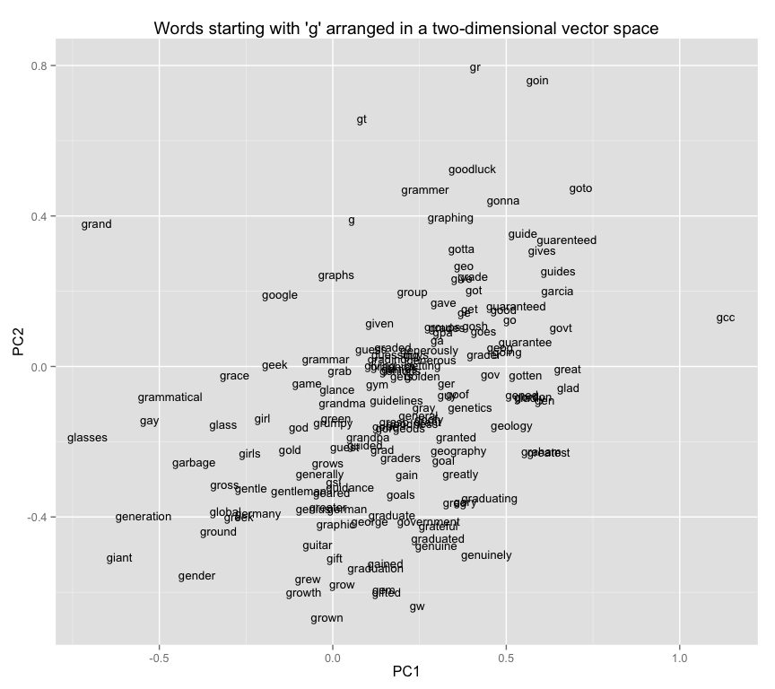
If you look at this plot, you’ll see that there are a lot of pairings where words with similar meanings are nearby. “Girl” is near “girls” and not all that far from “guy” and “guys”; “gonna” and “gotta”, which clearly have something in common, are next to each other; “green” and “gold,” the two colors, are relatively near to each other.
On the other hand, there’s a lot of junk. Why is “golden” far from “gold”? Maybe you can explain why “grumpy” is between “grandpa” and “grandma,” but why “gym?” If you’ve ever tried to read a network diagram, you’ve encountered a lot of strange juxtapositions like this, because two dimensions is simply not enough to capture broad relationships. You’d want the closest word to “grandma” to be “grandpa”, not “gym.” But there’s no single system of ranking where that happens automatically.
This isn’t entirely the fault of PCA. There more than two or three types of relationships in the world. “Mother” is like “father” except it’s female; like “grandmother” except it’s a generation removed; like “Mom” except that it’s more formal. Each of those express a different type of relationship. The goal of a perfect WEM transformation (something that doesn’t exist) is a vector space that can encode all of those relationships, simultaneously.
An R package for creating and exploring WEMs
The biggest is that they don’t have the instant gratification of one single display that summarizes their contents. I have printed out the top words in each topic of a model and brought it into a classroom: a WEM can’t fit onto a piece of paper like that.
At best it lets us reduce the vocabulary down into a two dimensional space like an improved word cloud.
Above is an example of such a plot based on one reduction of the dimensional space. It shows a number of clusters of similar words, though little overall structure. Terms that appear together (like “United” and “States”, “May” and “July”, or “yesterday” and “today”) cluster together on the chart. These plots have advantages over wordclouds, where position is completely meaningless: but they aren’t much more than a list of words.
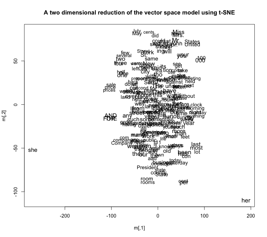
As a reductio ad absurdam, here’s a plot of the top 500 “words” in the Chronicling America set reduced into 3 dimensions. (This requires a webgl enabled browser and both dragging and zooming with the mouse before you can extract the full measure of confusion out of the visualization.) Three dimensions is better than two, but still not enough to discern meaning out of the directions. There are some notable patterns, though: there’s one cloud of numbers, there are various words plotted near each other, and so forth.
To really see what’s going on, you need to have ways of interacting with the vector space in far more dimensions than can be visualized. And therein lies the biggest hurdle for humanists using Word2Vec. Any form of interaction requires reductions and rotations of a space that can be hundreds of dimensions using techniques that draw on the basics of things like matrix multiplication, cosine similarity, and dot products. WEMs are fast and useful for data exploration precisely because they draw on a heritage of matrix-based computing that goes back to the good old days of FORTRAN. But most humanists don’t want to worry too much about the internals of linear algebra.
The wordVectors R package I’m putting up bundles the most basic operations you might want to do. It has two basic parts:
Functions to train a WEM using the original Word2Vec code and R wrappers by Jian Li (from the package
word2vec).Functions to read an existing WEM into R and then analyze it. I’ve written a number of convenience functions and object oriented syntax for some of the most useful operations you might perform the actual vector space that a WEM puts out. So the basic operations of a vector space model can be expressed through straightforward arithmetic. You’ll see some examples of this code below.
Getting started
So: what does it mean to represent a word as a vector? The idea is that each word gets a series of scores that position it in an arbitrary space. Rather than just one or two dimensions, which don’t allow many different relationships, this space has dozens or hundreds. (The two models I’ll be exploring here have 500 dimensions each.) That’s a lot; but it’s not nearly as many as the total number of documents, which is often the most sensible alternative, but is too large to be easily tractable on a computer.
So let’s get started by loading in a WEM representation. There are several floating around online: you can also train your own against a single file or folder of text files by using the wordVector function train_word2vec().
The vectors package gives an easy syntax using double brackets for denoting the vector represented by a word: “the vector representing”Democratic”, you enter chronam_vectors[["Democratic"]]. They work well with the feed-forward notation of the magrittr package, which I’ll be using below. If you know the Hadleyverse in R, you get it: if you don’t understand code at all, it should be as clear as anything else. Otherwise, think of the %>% symbol as a feed forward pipe from the command line.
Finding similar words.
One very basic operation is to find similar words. This can be quite useful in an information retrieval context. If you’re searching for a term, you should know what other words are related to refined your search; if you’re plotting words in Ngrams or Bookworm, you need to know what other synonyms might exist to see the difference between them.
So here are some examples. In each case, we take the full set of vectors, and then ask it for the nearest words to the vector defined by the vectors of a single word.
chronam_vectors %>% nearest_to(chronam_vectors[["judge"]]) %>% round(3)
##      judge     judges magistrate      Judge    justice       udge
##      0.000      0.329      0.361      0.378      0.412      0.414
##      bench      court    supreme     lawyer
##      0.423      0.423      0.430      0.440
The closest words to “judge” are all legal terms: the bench, the court, lawyer. The only odd element is the word “udge”; but remember, Chronicling America is one of the messiest sources of text out there, so common OCR misreadings should be close. How close, is a difficult question.
chronam_vectors %>% nearest_to(chronam_vectors[["oysters"]]) %>% round(3)
##  oysters    clams    crabs     fish   oyster  lobster     flsh   salmon
##    0.000    0.165    0.199    0.251    0.256    0.268    0.273    0.331
## mackerel    fried
##    0.351    0.359
Oysters is another nice example of a word that means something: everything that appears is related to seafood except for “fried.” (And another OCR error, “flsh.”)
chronam_vectors %>% nearest_to(chronam_vectors[["funny"]]) %>% round(3)
##     funny   comical laughable   amusing     queer     jokes ludicrous
##     0.000     0.217     0.248     0.264     0.270     0.275     0.295
##     laugh  humorous       fun
##     0.303     0.325     0.333
“Funny” works too. The four closest words are straightforward synonyms: “comical,” “laughable”,“amusing”, and “queer.”
Not everything works perfectly. Particularly common words get lost: here are the closest words for “new” and “good.” After a point, the OCR errors start to dominate; and almost anything, evidently, can appear in the context of “new.”
chronam_vectors %>% nearest_to(chronam_vectors[["new"]]) %>% round(3)
##      new      now     This complete        A    large       in        -
##    0.000    0.412    0.441    0.468    0.488    0.489    0.489    0.492
##     only     fine
##    0.492    0.493
chronam_vectors %>% nearest_to(chronam_vectors[["good"]]) %>% round(3)
##     good     pood     Rood     gcod     fine     gocd splendid     eood
##    0.000    0.274    0.287    0.316    0.329    0.334    0.352    0.361
##     best     sood
##    0.362    0.379
Exploring thematic clusters.
Just similarity metrics start to open up some interesting opportunities for exploration. Similarity isn’t just a way to finding nearest words: it’s also something can extract out items of a single class. You could think of this as a supervised form of topic modeling: it lets you assemble a list of words that typically appear in similar contexts. But instead of letting the algorithm choose a fixed number of topics, WEMs let you choose how expansive you want the explored space to be.
Since I already typed in “oysters”, let’s take food as an example. In topic modeling, you run a model and hope that a “food” topic emerges. To get a list of foods in a working WEM, you can just start from something that you know to be food to begin with.
First we need some different types of food. Just “oysters” as a descriptor isn’t great: I’ll start by seeding the search with a few different food words.
chronam_vectors %>% nearest_to(chronam_vectors[[c("oysters","ham","bread","chicken")]],20) %>% names
##  [1] "fried"      "oysters"    "chicken"    "soup"       "bread"
##  [6] "roast"      "baked"      "hash"       "lobster"    "cooked"
## [11] "meat"       "sandwich"   "stew"       "pudding"    "gravy"
## [16] "sandwiches" "mince"      "salad"      "biscuits"   "dish"
The easiest way to explore these spaces is just to work iteratively until you get a vector that seems good enough. I’ll add some of the words I like from the bottom half of that search to get us towards something even more food-y. I’m doing this a few times, until we get out to about 300 words: the list below just shows 50 random words out of that set.
food_words = chronam_vectors %>% nearest_to(chronam_vectors[[c("oysters","ham","bread","chicken","sausage","cheese","biscuits","peanut","sardines","squash","peaches","cherries","berries","kale","sorghum","tomatoes","asparagus","lima","egg","steak","salmon","mackerel","shad")]],300) %>% names
sample(food_words,50)
##  [1] "stalk"       "relish"      "loaf"        "kale"        "Cabbage"
##  [6] "veal"        "dish"        "roast"       "berry"       "sandwich"
## [11] "almond"      "cans"        "evaporated"  "seedless"    "cinnamon"
## [16] "carp"        "baked"       "dishes"      "jam"         "currants"
## [21] "toast"       "sieve"       "milk"        "grape"       "gravy"
## [26] "freshly"     "veg"         "varieties"   "cocoanut"    "eels"
## [31] "boiled"      "honey"       "ham"         "tomatoes"    "Squash"
## [36] "saucepan"    "mush"        "canning"     "slice"       "lamb"
## [41] "peel"        "pound"       "basket"      "pickled"     "watermelons"
## [46] "turkey"      "cake"        "bbL"         "smoked"      "lard"
Now we have a bunch of food words typical of late-19th century newspapers. (You notice that many of them are instructions: that’s because food in newspapers is largely about recipes. Reprinted recipes are one of the major sets of clusters in my colleagues’ Ryan Cordell and David Smith’s Viral Texts Project.) We can use similarity scores for all sorts of things. We can, for instance, create a hierarchy of food words based on their distances from each other.
foods = chronam_vectors[rownames(chronam_vectors) %in% food_words[1:50],]

food_distances = cosineDist(foods,foods) %>% as.dist
plot(as.dendrogram(hclust(food_distances)),horiz=F,cex=1,main="Cluster dendrogram of the fifty words closest to a food vector\nin newspapers from Chronicling America")
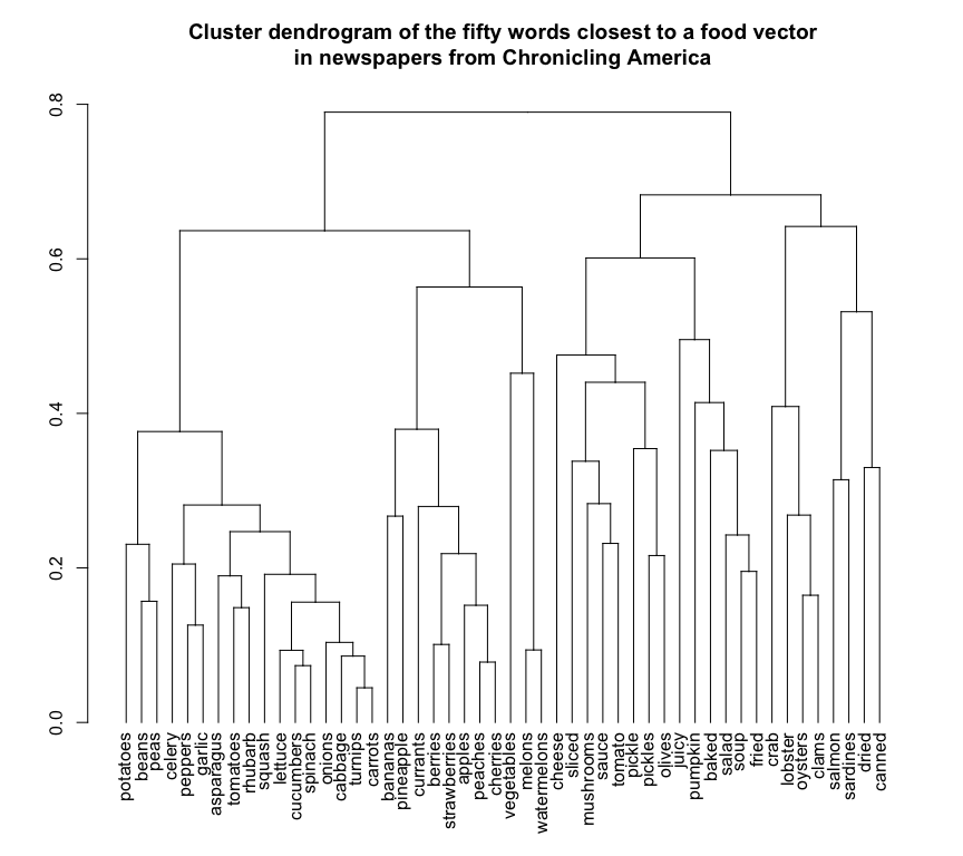
Cut at about .6, and this clustering seems to be properly segregating off with just one or two errors vegetables, fruit, seasoning/cooking, and fish. (There’s an error here, too: meat products don’t appear at the heart of the food cluster. Maybe because they’re also animal names, or because they get traded on the commodity markets, or something. Grains are also missing, which share the same distinguishing features.)
We can also pull out similarity scores for all words in the set to either of two terms: a meat vector and a vegetable vector: this lets us plot a number of food terms in a discursive space vaguely defined as “meatness” and “vegetableness.” (Meatspace, as it were.)
foods = chronam_vectors[rownames(chronam_vectors) %in% food_words,]
meat_score = foods %>% cosineSimilarity(chronam_vectors[[c("meat","meats")]])
vegetable_score = foods %>% cosineSimilarity(chronam_vectors[[c("vegetable","vegetables")]])

plot(meat_score,vegetable_score,type='n',main="Top 300 food words plotted by their similarity to meats\n(x axis) and vegetables (y axis).")
text(meat_score,vegetable_score,labels=rownames(foods),cex=.7)
abline(a=0,b=1)
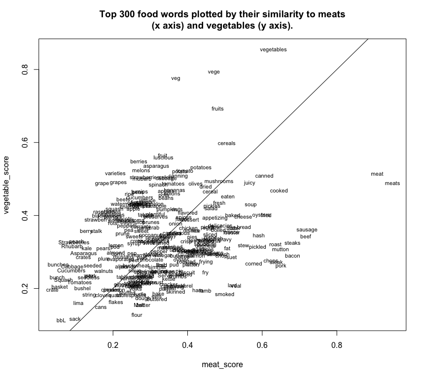
High vegetable scores are towards the top, and high meat scores towards the right; to the top/left of the line are words more like vegetables, and to the bottom/right are words more like meats. There are some vaguely surprising things for me in here: that “pickled” is so strongly associated with meats.
But what’s really powerful, and I’ll get into more in a second, is that we don’t need two dimensions to capture the meat-vegetable relationship: we can do it in one. Just as “meat” is a vector and “vegetable” is a vector, “meat”-“vegetable” is also something that we can track in space. In the text_vectors package, we can simply indicate this by comparing our words to a new vector defined as chronam_vectors[["meat"]] - chronam_vectors[["vegetable"]]
This is a relationship, not a vocabulary item: but it is defined in the same vector space, so we can score any words based on their relationships to it.
This means we can create text layouts specific to any desired word relationship.
If that relationship is so important that it makes its way into the model’s outputs, we can see it in action.
all_foods = data.frame(word = rownames(foods))

meat_vegetable_vector = chronam_vectors[["meat"]] - chronam_vectors[["vegetable"]]

all_foods$meatiness_vs_veginess = cosineSimilarity(foods,meat_vegetable_vector)

sweet_salty_vector = chronam_vectors[[c("sugar","sweet")]] - chronam_vectors[[c("salty","salt")]]

all_foods$sweet_vs_salty = cosineSimilarity(foods,sweet_salty_vector)

library(ggplot2)
ggplot(all_foods,aes(x=meatiness_vs_veginess,y=sweet_vs_salty,label=word)) + geom_text(size=2.5) +
  scale_y_continuous("<----- saltier ..............  sweeter ------>",limits=c(-.45,.25)) +
  scale_x_continuous("<----- vegetalier ..............  meatier ------>",limits=c(-.25,.33))
## Warning: Removed 5 rows containing missing values (geom_text).
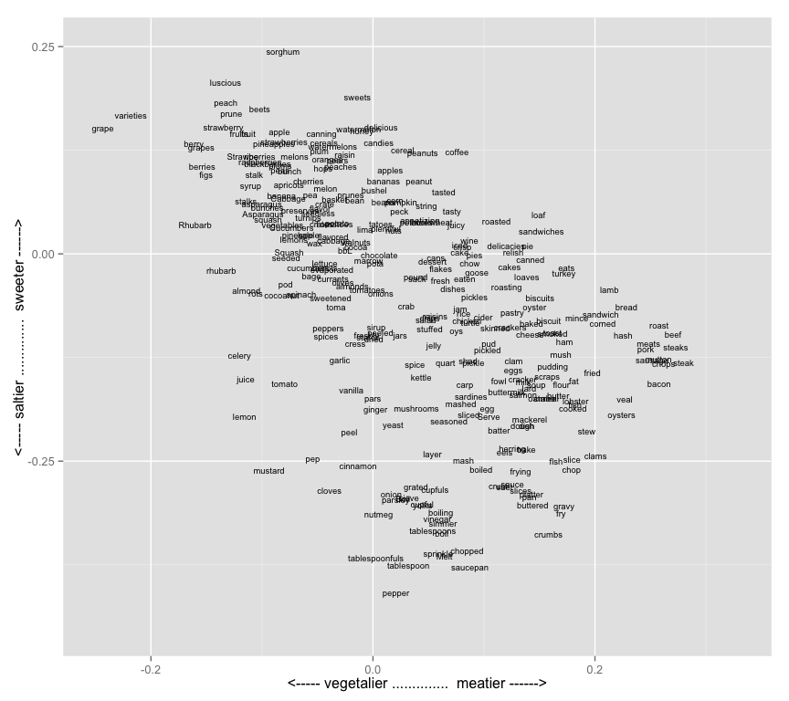
The dimensions here appear to me to be capturing some useful distinctions about food prepartion practices in the United States between 1860 and 1922. The foods generally drift down and to the right because saltiness and meatiness are correlated. But in the deviations lie distinctions in the way certain foods are prepared. Lamb and poultry are the meats most associated with sweet/sugary preparations or results; lemon, celery and tomato the fruits/vegetables most associated with salt. Frying and boiling are methods of preparation that incline towards saltiness; roasting and canning with sweetness. And so forth.
This is, obviously, something of a toy example; I don’t know enough about late-19th-century food to necessarily see what’s interesting here. I go into the food example not because I’m trying to produce substantive answers to historical questions, but to show the ways that a method like this operates.
The point, though, is that that “sweet/salty” and “vegetable/meaty” are both binary relations that share some interesting properties:
They are not captured by a single word;
They nonetheless exist, in some sense, in the real world;
They exist as a spectrum rather than a class.
I don’t think it’s a stretch to say that most interesting problems in the humanities are this sort of thing. When we study the discourse of Catholicism, we tend to actually mean not some abstract linguistic field on its own but rather a set of vocabularies in tension with other ones. One person might study Catholic rhetoric compared to protestantism; another compared to atheist rhetoric; another compared to indigenous cultures.
Less flexible data models like topic models lock you into one particular idea of what Catholicism, or food, or any other topic, might be. WEMs, on the other hand, explicitly enable searching for relations embedded in words. If there’s a binary, it’s open for exploration. Lamb isn’t that associated with sweetness, but is sweet for a meat; celery isn’t salty, but tends to show up with salt a lot for a vegetable.
This doesn’t mean that “meatiness/vegetaliness” is a topic that the model learned: instead, it means that certain aspects of the differences between meats and vegetables are things that emerge out of reading a large corpus like this. Vegetables appear near “green,” meats appear near “brown,” and so forth: and that some shadow of that actual semantic relationship managed to appear in the data.
Now, I know no one who studies “meatiness” as a binary. But a tremendous number of humanities projects are constructed around things that can be conceived as binaries. Center/periphery,prestigious/popular, protestant/catholic, etc.; toying with with implications of some binary in language is at the heart of all sorts of humanistic work. I’ll write a bit about the gender binary in a little bit, because I think it’s an excellent example of how looking for the expression of a binary can help us to understand social forces at work, even when that’s a binary that most recent work in the field is more interesting in deconstructing than reifying.
So one the core research strategy for word2vec is: are you interested in the behavior of language across some semantic space that could be characterized as a binary relationship between words or groups of words? If so, you may be able to drop the tool into your workflow.
Analogy
I would be remiss if I didn’t mention one other thing in my introductory post.
The purest form of relationship is analogy. This is one of the great strengths of WEMs. As the author of word2vec says, one of the most fascinating features is that the word-vector space preserves semantic relationships
It was recently shown that the word vectors capture many linguistic regularities, for instance vector operations
vector('Paris') - vector('France') + vector('Italy')results in a vector that is very close tovector('Rome'), andvector('king') - vector('man') + vector('woman')is close tovector('queen').
Here’s a video representation of that from @ericcolson on Twitter
https://pbs.twimg.com/tweet_video/CDd60dUUkAAEXLt.mp4
The classic queen-king example works neatly with the historical newspaper data: the female equivalent of “king” is “queen.”
nearest_to(chronam_vectors,chronam_vectors[["king"]]-chronam_vectors[["man"]]+chronam_vectors[["woman"]],5) %>% round(3)
##    queen     king   prince   throne princess
##    0.196    0.211    0.322    0.325    0.325
Many of the newspaper corpora from the last 20 years work well at capital cities tasks as well. The Chronicling America set, at least as I have trained it, is not so good at geographical reasoning. It thinks the capital of Georgia is Richmond, not “Atlanta,” or that the London of France is London, not Paris.
nearest_to(chronam_vectors,chronam_vectors[["Richmond"]]-chronam_vectors[["Virginia"]]+chronam_vectors[["Georgia"]],5)
##  Richmond   Georgia   Augusta        Ga     Macon
## 0.3677742 0.3803775 0.4208831 0.4390361 0.4528889
nearest_to(chronam_vectors,chronam_vectors[["London"]]-chronam_vectors[["England"]]+chronam_vectors[["France"]],5)
##    London     Paris    Berlin    France     ondon
## 0.2314020 0.2656150 0.2922507 0.3141335 0.3763772
Some of these are sensible. If we construct a vector that averages out a number of different capital relationships, things work better. I’m constructing these vectors as two lists: one is the average of a number of major cities, and the second is the
major_cities = chronam_vectors[[c("London","Berlin","Moscow","Vienna")]]
countries = chronam_vectors[[c("England","Germany","Russia","Austria")]]
nearest_to(chronam_vectors,major_cities - countries + chronam_vectors[["France"]],5)
##     Paris    Berlin    Vienna    France    London
## 0.1765068 0.2106330 0.3109084 0.3140178 0.3365720
nearest_to(chronam_vectors,chronam_vectors[[c("Austin","Cleveland","Hartford","Harrisburg","Phoenix")]]-chronam_vectors[[c("Texas","California","Connecticut","Pennsylvania","Arizona")]]+chronam_vectors[["Georgia"]],5)
##    Georgia    Augusta Charleston      Macon     Gaines
##  0.2746897  0.3974189  0.4181139  0.4251169  0.4341202
Along the same lines: in the Rate My Professor dataset, which includes more information about academic classes, we can look for the words closest to “hola.”
teaching_vectors %>% nearest_to(teaching_vectors[["hola"]])
##          hola       espanol         todos    fantastico        porque
## -4.440892e-16  5.419217e-01  5.561170e-01  5.582298e-01  5.584173e-01
##   interesante          buen     simpatico           muy     profesora
##  5.646364e-01  5.702220e-01  5.703893e-01  5.707483e-01  5.709447e-01
That gives us a bunch of Spanish-language words. Suppose we subtract out the vector for “spanish” from that?
Remarkably, the top matches (after hola itself) are several words that roughly mean “hello” in English: “hi”, “goodmorning”, “wassup”, and “hello.”
teaching_vectors %>% nearest_to(teaching_vectors[["hola"]]-teaching_vectors[["spanish"]])
##        hola          hi goodmorning    mmmmmkay      wassup       hello
##   0.2541650   0.6992011   0.7123197   0.7195401   0.7225225   0.7289345
##       todos         uhm   hahahahah        quot
##   0.7447951   0.7485577   0.7516170   0.7620057
Add “French” into the mix, and now “bonjour” floats to near the top of the list.
teaching_vectors %>% nearest_to(teaching_vectors[["hola"]] - teaching_vectors[["spanish"]] + teaching_vectors[["french"]],n=5)
##      hola   bonjour    french    revoir    madame
## 0.1282269 0.5520502 0.6021849 0.6156018 0.6170013
So what’s going on here? It’s not really translating languages, but instead is telling us about what words occupy similar slots. So when we subtract “spanish” out, we’re saying “what words do people use in similar situations to ‘ hola ’, not including similarities that appear in the context of”spanish”? “Hola” can be used in English as well as in Spanish; my sense is that it acts as a particularly informal greeting. So maybe it makes sense that “wassup” takes the same place.
The point is: the vector arithmetic works reasonably well at turning up unexpected but plausible solutions for a variety of queries. For toying around with a large corpus to see what makes it tick, this is one of the most valuable things we can have.
Can analogies lead to new information?
These particular examples tend to make machine learning algorithms look simpleminded if you’re not already invested in analogy tasks. Of course a king is a male queen! If it can’t accurately find either the capital or the most important city in Georgia, what can it do?
So let’s try a less trivial example. Remember, these algorithms only know things based on the corpus they’re trained on. Testing for major cities may be difficult because the Chronicling America set is composed of a non-representative set that includes many small-town newspapers; some of those may be confusing the algorithm.
The Rate My Professor corpus contains a lot of information about what goes on inside classrooms. I’m curious what textbooks are being assigned. Can we use just student evaluations of professors to find the dominant textbook author in an academic discipline today?
To start, we need a seed piece of knowledge. So, I happen to know that Greg Mankiw wrote the most widely used introductory economics text. Now I’ll ask what word is closest to the analogous position to the word “history” that “mankiw” occupies relative to “economics”.
There is one problem here: it thinks that “mankiw” himself is in that slot. This is a sign we’re asking a non-perfectly clear question for the model: the two query words are the closest, which means the vector separating it is relatively short. But if we ignore “mankiw” and “history”, the terms used in constructing the query, it correctly answers that Eric Foner wrote the leading introductory history textbook.
teaching_vectors %>% nearest_to(teaching_vectors[[c("mankiw")]] - teaching_vectors[[c("econ","economics")]]+teaching_vectors[[c("history","hist")]],15)
##          mankiw            hist         history           foner
##       0.2424912       0.5402814       0.6234560       0.6278997
##          author      historians        authored       historian
##       0.6464106       0.6575385       0.6648746       0.6806184
##         primary            text          takaki      sourcebook
##       0.6864897       0.6874832       0.6907583       0.6927253
##      publishers         authors chronologically
##       0.6958308       0.7008529       0.7030050
That’s our confirmation step: I already know that Foner is the leading US History text. I don’t know who wrote the leading chemistry text: let’s give it a shot.
According to this, McMurry wrote a leading chemistry textbook. That seems to be true. Here the noise gets louder, though. Is ACS (the American Chemical Society) a textbook author? Maybe; maybe not.
textbook_authorship_vector=teaching_vectors[[c("mankiw")]] - teaching_vectors[[c("econ","economics")]]

teaching_vectors %>% nearest_to(textbook_authorship_vector+teaching_vectors[[c("chem","chemistry")]])
##    mankiw      chem   organic chemistry     ochem      orgo       chm
## 0.2542234 0.5104880 0.5409168 0.5543635 0.5756683 0.5823762 0.5930418
##       acs       owl   mcmurry
## 0.5932805 0.6062949 0.6132635
Physics turns up “Tipler,” which is a plausible guess, at least if you suspend the requirement that it be the leading textbook and just let it be “some physics textbook.”
teaching_vectors %>% nearest_to(textbook_authorship_vector+teaching_vectors[[c("physics")]])
##           mankiw          physics        webassign        mastering
##        0.2430949        0.5304092        0.6101680        0.6123962
## masteringphysics     smartphysics           tipler         cramster
##        0.6316525        0.6326244        0.6573281        0.6592712
##              phy          mcmurry
##        0.6746490        0.6749715
But for biology and pyschology, there’s no textbook authors in sight.
teaching_vectors %>% nearest_to(textbook_authorship_vector + teaching_vectors[[c("bio","biology")]])
##           mankiw              bio          biology             biol
##        0.2192941        0.5265739        0.5675650        0.5948005
##       physiology         genetics masteringbiology          zoology
##        0.6376425        0.6458629        0.6532397        0.6568374
##          anatomy         microbio
##        0.6620395        0.6632609
teaching_vectors %>% nearest_to(textbook_authorship_vector+teaching_vectors[[c("psych","psychology")]])
##        mankiw         psych    psychology      abnormal           psy
##     0.2372132     0.5533798     0.5606939     0.5836853     0.6101105
##  psychologist          psyc      lifespan psychologists         pysch
##     0.6271077     0.6421404     0.6462094     0.6480856     0.6574128
teaching_vectors %>% nearest_to(teaching_vectors[[c("mankiw")]] - teaching_vectors[[c("econ","economics")]]+teaching_vectors[[c("botany")]])
##       mankiw       botany      zoology   vertebrate        plant
##    0.3001308    0.4043690    0.5927225    0.6038217    0.6068790
##       plants      ecology         biol  systematics invertebrate
##    0.6068897    0.6141464    0.6169070    0.6170955    0.6228298
Still, this is fairly remarkable. “Foner” only appears 19 times in the corpus: “Mankiw”, 42. For them to appear properly associated with their native disciplines and as textbook authors is testament to the ability of the algorithm to pick up fairly quickly on significant patterns.
The lesson from this may be that this method has the potential to produce possible avenues, as much as it does to solve questions. For search-type queries like these, that is an appropriate outcome. The predominant test of these methods in the machine-learning world are to make sure that machines can accurately answer these individual queries. For most humanistic results, it may be that one suggestive lead inside five dead-ends is as good as anything else.
The real value of these analogies, though, I’ll hold off for arguing in a separate post: they can help us identify words that show unusual patterns along any arbitrary dimensions.
Some other examples
Let me finish up with just a few other notes that may be of technical interest to a few people.
Polysemy
Polysemy is the existence of multiple meanings for the same word. Topic models tend to handle polysemy by noticing that a word appears in multiple contexts, and assigning a word to different topics.
With simple nearest neighbor approaches, WEM models seem to lack a sense of the multiple meanings of words. For example, if ask for nearest words to “bank” in the ChronAm set, we get a number of words that relate to the banking industry and none that relate to the shore of a river.
chronam_vectors %>% nearest_to(chronam_vectors[["bank"]])
##         bank         hank       bank's        banks      cashier
## 2.220446e-16 1.827868e-01 2.778337e-01 3.353049e-01 3.434093e-01
##         Hank         bunk      defunct    depositor   depositors
## 3.517692e-01 3.578958e-01 3.758841e-01 3.778528e-01 3.779416e-01
We can see this in the cosine similarity metrics. “Bank” has a similarity to “river” and “shore” of roughly 0.2, but a much higher similarity to “depositor” and “cashier” of about 0.6.
chronam_vectors %>%
  filter_to_rownames(c("river","shore","depositor","cashier")) %>%
  cosineSimilarity(chronam_vectors[["bank"]])
##                [,1]
## river     0.2749651
## shore     0.1242357
## cashier   0.6565907
## depositor 0.6221472
One solution to polysemy is to simply use the project of vector rejection to eliminate a meaning from a word. In the following image from Wikipedia, you can think of vector A as the word “bank” and vector B as meaning “the banking system”, generally. Most of the vector for the word “bank” (a1) lies parallel to A; but some portion (a2) is completely perpendicular.

Vector Rejection
We can extract a vector, though, that means “bank not in the sense of a depository institution” by using a process of vector rejection. Rejection is the opposite of projection: it finds the portions of a vector that are not parallel to a given vector. This is such a basic operation that I’ve built it into the TextVectors package as the function reject(matrix,orthogonal_vector).
By removing the proportions of “bank” that are parallel to words having to do with the banking industry, we can create a vector that gives us words related to riverbanks and, it turns out, the situation of towns (on roads, in districts, “lying” places, and so forth.)
financeless_bank = chronam_vectors[["bank"]] %>%
             reject(chronam_vectors[["cashier"]]) %>%
             reject(chronam_vectors[["depositors"]]) %>%
             reject(chronam_vectors[["check"]])

chronam_vectors %>% nearest_to(financeless_bank)
##      bank     river     banks      side      road      live      lies
## 0.6034296 0.7017586 0.7320919 0.7455139 0.7463685 0.7495098 0.7540568
##     still  district       tha
## 0.7559630 0.7563237 0.7594058
It’s worth noting that this works primarily because it strips away the other meanings: the new vector only slightly more similar to “river” than the old one.
chronam_vectors[["bank"]] %>%
       cosineSimilarity(chronam_vectors[["river"]])
##           [,1]
## [1,] 0.2749651
chronam_vectors[["bank"]]  %>%
             reject(chronam_vectors[["cashier"]]) %>%
             reject(chronam_vectors[["depositors"]]) %>%
             reject(chronam_vectors[["check"]]) %>%
      cosineSimilarity(chronam_vectors[["river"]])
##           [,1]
## [1,] 0.2982414
Still, this opens up some interesting possibilities for exploring the dominant meanings of words in a single large corpus. In word-analysis platforms like Bookworm or Ngrams, we often do not know the different senses a word might take. Further analysis of the various different spaces a vector takes up might be useful at starting to show some potentially different meanings.
On the other hand, the most naive approaches to this do not work especially well. Using hierarchical clustering, for example, the “river” sense becomes naturally entangled with “railroad” and “road”, which then associates itself a bunch of words in the area of political economy. So the model is not great at decomposing into individual meanings.
Which vector-space representation to use?
I’m using here the outputs of Word2Vec, which kick-started this particular branch of research in 2012. (2013?) GloVe offers the same kind of output, a sounder theoretical justification of what the vectors mean, roughly comparable performance on analogy tasks, and a few trade-offs in terms of training difficulty. One major advantage of GloVe is that it can work more efficiently on an intermediate precomputed stage: that means that for work that involves building a variety of models and comparing them to each other, GloVe may be a better choice. (This might hold, for instance, with Bookworm or JStor DFR sets where it is desirable to train several models on metadata corpora and see how they differ.)
In general, word2vec takes longer to train but requires less memory; GloVe takes less time but requires more memory. I use word2vec in part because I find it easier to use for training a document with a defined vocabulary, but mostly because it seems easier to integrate with Bookworm using the online gensim implementation of the algorithm.
There is some question whether the newer word embeddings adds a great deal over other more traditional NLP at all. The argument for using it in the digital humanities, as I see it, is not that the results are necessarily better than any other constellation of dictionaries and treebanks, but, as Levy et al. put it in a paper somewhat critical of word2vec, its basic defaults (skip-grams, SGNS in the negative paragraph below) work fairly well across a variety of situations. “Out of the box,” as it were, a standard skip-gram model can provide decent results.
SGNS is a robust baseline. While it might not be the best method for every task, it does not significantly underperform in any scenario. Moreover, SGNS is the fastest method to train, and cheapest (by far) in terms of disk space and memory consumption.
Current projects using word2vec
In DH
(Let me know in the comments what I’m missing)
Possibly I’m just not paying attention, but I haven’t seen all that much exploration of word2vec out there by non-computer-scientists in the digital humanities. Here are a few.
Alan Liu’s page here says they have ‘ buzz ’.
Melvin Wevers has used multiple multiples from different years as a way of tracing the shifting meaning of a single word. The University of Amsterdam seems to have a few interesting projects using the methods, in general.
Doug Duhaime has outlined the use of pre-trained GloVe vectors for creating vocabulary clusters.
Scott Enderle has proposed that the skip-gram model may make sentences susceptible to calculus because of type theory. I don’t really understand what that means, but doesn’t it sound fun?
Lynn Cherny has experimented with visualizing word embeddings for Jane Austen novels.
Elsewhere
(Non-comprehensive, just what I’ve found useful.)
The gensim python implementation is excellent. I’m using it rather than Mikolov’s C code for the Bookworm word2vec implementation because it handles streaming data better.
Radim Rehurek, the author of gensim, also has an introduction to word2vec’s algorithm and debates over it that is the clearest and most useful I’ve seen.